NEON tick pathogen data
Sara Paull 2023-05-09
Data Descriptions
NEON is generating a unique group of complimentary datasets to improve understanding of the mechanisms underlying tick-borne pathogen transmission.
Tick collection using drag cloths occurs every 3-6 weeks at 47 terrestrial field sites. Ticks are collected and stored in 95% ethanol. Following collection, tick samples are sent to a professional taxonomist where ticks are identified to species, and life-stage (or sex if adults). A subset of positively-identified nymphal ticks of the species Ixodes scapularis and Amblyomma americanum have been tested for the presence of bacterial and protozoan pathogens. Data collection began at some sites as early as 2014, with all sites having data beginning in 2019.
Small mammal box-trapping occurs 4-6 times per year at 3-8 grids across 44 terrestrial field sites. Several different types of samples are collected from target taxa including ear and blood samples. Small mammal data collection began at some sites as early as 2014, with all sites having data beginning in 2019. Beginning in 2020, a subset of blood samples have been tested for several bacterial tick-borne pathogens. The ear samples in all regions within and bordering areas where Lyme disease has been detected have been tested for Borrelia burgdorferi.
require("neonUtilities")
require("dplyr")
require("ggplot2")
#Select the dates and sites for data download:
sd = '2021-01'
ed = '2022-01'
sites = c("SCBI", "HARV", "TREE")

#download ticks sampled using drag cloth
tckColl <- loadByProduct(
  dpID='DP1.10093.001',
  startdate = sd,
  enddate = ed,
  site = sites,
  package='basic',
  check.size = F)

#download tick pathogen status
tckPath <- loadByProduct(
  dpID='DP1.10092.001',
  startdate = sd,
  enddate = ed,
  site = sites,
  package='basic',
  check.size = F)

#download small mammal trapping data
mamColl <- loadByProduct(
  dpID="DP1.10072.001",
  startdate = sd,
  enddate = ed,
  site=sites,
  package="basic",
  check.size = F)

#download rodent pathogen tick-borne data
mamPath <- loadByProduct(
  dpID="DP1.10064.002",
  startdate = sd,
  enddate = ed,
  site=sites,
  package="basic",
  check.size = F)
#Separate the downloaded lists into dataframes for ease of accessing data tables:
list2env(tckColl, envir=.GlobalEnv)
list2env(tckPath, envir=.GlobalEnv)
list2env(mamColl, envir=.GlobalEnv)
list2env(mamPath, envir=.GlobalEnv)
#Calculate pathogen prevalence for ticks:
tpp<-tck_pathogen %>%
  mutate(taxonID = substr(testingID,19,24)) %>%
  group_by(siteID, testPathogenName, taxonID) %>%
  summarise(tot.test=n(), tot.pos = sum(testResult=='Positive')) %>%
  mutate(prevalence = tot.pos/tot.test)

#Calculate pathogen prevalence for mammals:

#First split the rodent pathogen data by sample types (ear or blood) before joining
# with the trapping data in order to get the taxonID of the small mammal from which
#the samples were taken (there are 2 different columns for sampleID in
# the mammal trapping data - one for blood samples and one for ear samples)
rptear<-rpt2_pathogentesting %>% filter(grepl('.E', sampleID, fixed=T))
rptblood<-rpt2_pathogentesting %>% filter(grepl('.B', sampleID, fixed=T))

#Join each sample type with the correct column from the mammal trapping data.
rptear.j<-left_join(rptear, mam_pertrapnight, by=c("sampleID"="earSampleID"))
rptblood.j<-left_join(rptblood, mam_pertrapnight, by=c("sampleID"="bloodSampleID"))
rptall<-rbind(rptear.j[,-75], rptblood.j[,-80]) #combine the dataframes

mpp<-rptall %>%
  group_by(siteID.x, testPathogenName, taxonID) %>%
  summarise(tot.test=n(), tot.pos = sum(testResult=='Positive')) %>%
  mutate(prevalence = tot.pos/tot.test) %>%
  rename(siteID = siteID.x)
Explore Lyme prevalence across sites and taxa
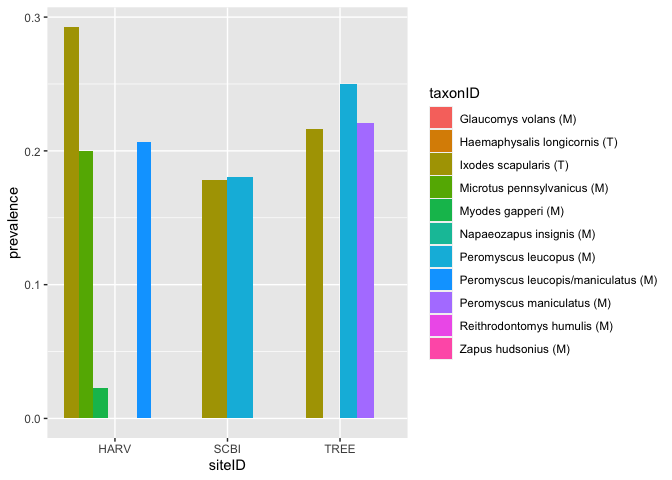
There is considerable interest in improving understanding of the factors that contribute to the spread of the bacterial pathogen, Borrelia burgdorferi, which causes Lyme disease. Here we make a simple barplot of the prevalence of this pathogen in 2021 in small mammals (M) and ticks (T) at 3 different sites.
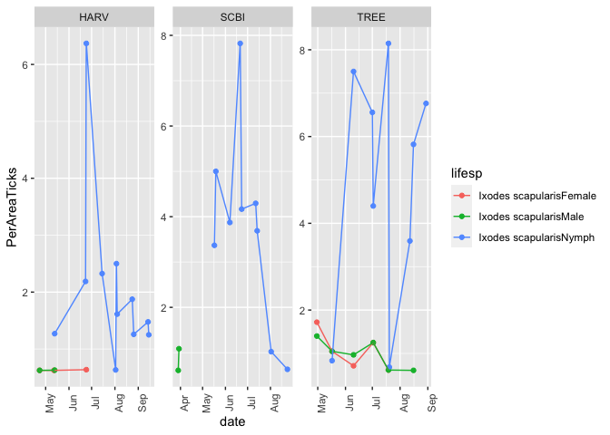
The abundance of ticks and small mammals found at a site likely plays a role in understanding the interplay between environment, hosts and vectors in this complex system. Here we plot the abundance of 3 life stages of the primary vector, Ixodes scapularis at the three selected sites. A more detailed tutorial describing how to get started analyzing and plotting small mammal abundances can be found here: https://www.neonscience.org/resources/learning-hub/tutorials/mammal-data-intro