Learn · Tutorial
2. Verbs do things
Concept
A verb factory configures an operation; the returned callable applies it to data. Run the shared setup first.
Tiny example
A factory such as v.mean(dim="time") configures a callable. A pipe applies
it to data. Here, follow the same temperature cube from a map to a selected
window, local departures, a regional summary, standardization and a saved result.
Explanation
The pipe changes Python calls to a readable analytical sentence; it does not change the mathematics. Each figure immediately follows its producing code. The mean reference documents reduction dimensions. Run this exact sequence in the grammar notebook.
Try it / worked example
REAL DATA · Reviewed local PRISM observations; no live request.
Reproduce: imports, checked data and setup
Run in a clone after python -m pip install -e '.[vignettes]'.
from pathlib import Path
import hashlib
import json
import numpy as np
import pandas as pd
import xarray as xr
import matplotlib.pyplot as plt
from IPython.display import display
from cubedynamics import pipe, verbs as v

# Run in the cloned repository or beside a downloaded notebook in the repo.
repo = next(p for p in (Path.cwd(), *Path.cwd().parents)
            if (p / "tests/fixtures/real_data").is_dir())

def observed_cube(stem, variable):
    path = repo / "tests/fixtures/real_data" / (stem + ".nc")
    record = json.loads(path.with_suffix(".provenance.json").read_text())
    assert hashlib.sha256(path.read_bytes()).hexdigest() == record["fixture_sha256"]
    with xr.open_dataset(path, engine="scipy") as dataset:
        assert not dataset.attrs["is_synthetic"]
        result = dataset[variable].load()  # Only this small, reviewed local extract.
        result.attrs = {**dataset.attrs, **result.attrs}
    assert result.dims == ("time", "y", "x")
    assert np.all(np.diff(result.x) > 0) and np.all(np.diff(result.y) < 0)
    assert bool(np.isfinite(result).all())
    return result

cube = observed_cube("prism_boulder_january_2024", "tmax").rename("temperature")
assert cube.attrs["units"] == "degC"

plt.rcParams.update({'font.family': 'DejaVu Sans', 'font.size': 12, 'axes.titlesize': 13, 'axes.labelsize': 12, 'figure.facecolor': 'white', 'axes.facecolor': 'white', 'savefig.facecolor': 'white', 'figure.dpi': 140})
Start with a temperature field
Where was the cold outbreak visible on 16 January?
field = cube.sel(time="2024-01-16")

fig, ax = plt.subplots(figsize=(5.4, 3.8), layout="constrained")
field.plot(ax=ax, cmap="magma", cbar_kwargs={"label": "Daily maximum (°C)"})
ax.set(title="PRISM · Boulder · 16 January 2024",
       xlabel="Longitude (°E)", ylabel="Latitude (°N)")
plt.show()
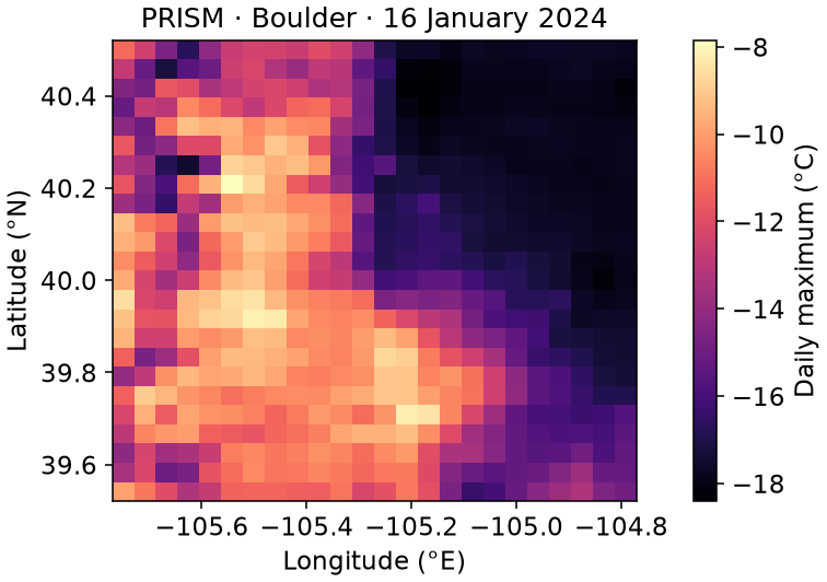
What changed? Each cell is a gridded estimate, not a station reading. This map shows absolute temperature; it does not yet say how unusual the day was.
Choose the time window
Which observations will define the short-period baseline?
window = (pipe(cube)
          | v.apply(lambda c: c.sel(time=slice("2024-01-10", "2024-01-20")))).unwrap()
assert window.sizes["time"] == 11

fig, ax = plt.subplots(figsize=(5.4, 3.4), layout="constrained")
cube.isel(y=12, x=12).plot(ax=ax, color="0.65", label="Full fixture")
window.isel(y=12, x=12).plot(ax=ax, marker="o", color="#246b70", label="Selected days")
ax.set(title="One grid cell · select 10–20 January", xlabel="Date", ylabel="Daily maximum (°C)")
ax.legend(frameon=False)
plt.show()
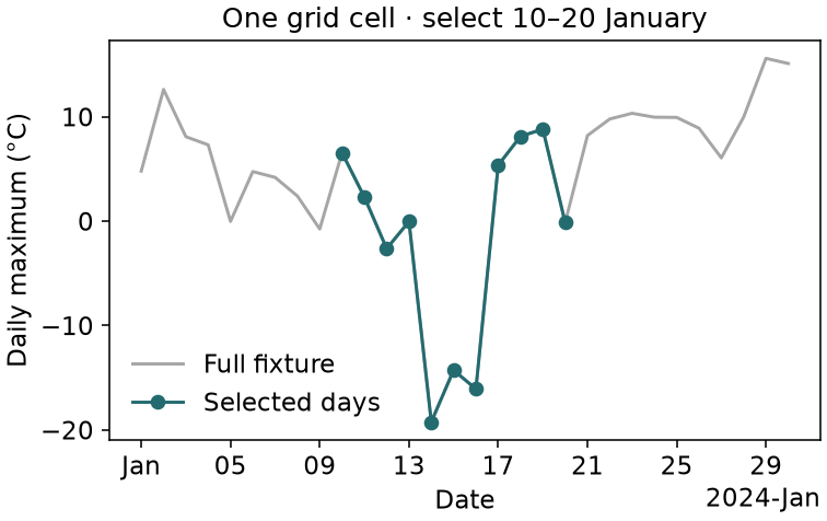
What changed? The grey observations remain in cube but not window. Subsequent anomalies use these eleven selected days, not the entire month or a climatology.
Remove the local baseline
Where was 16 January colder than each pixel’s own selected-period mean?
departures = (pipe(window) | v.anomaly(dim="time")).unwrap()

fig, axes = plt.subplots(2, 1, figsize=(5.4, 6.5), layout="constrained")
window.sel(time="2024-01-16").plot(ax=axes[0], cmap="magma", cbar_kwargs={"label": "°C"})
departures.sel(time="2024-01-16").plot(ax=axes[1], cmap="RdBu_r", center=0,
                                    cbar_kwargs={"label": "Departure (°C)"})
for ax, title in zip(axes, ["Before · absolute temperature", "After anomaly() · local departure"]):
    ax.set(title=title, xlabel="Longitude (°E)", ylabel="Latitude (°N)")
plt.show()
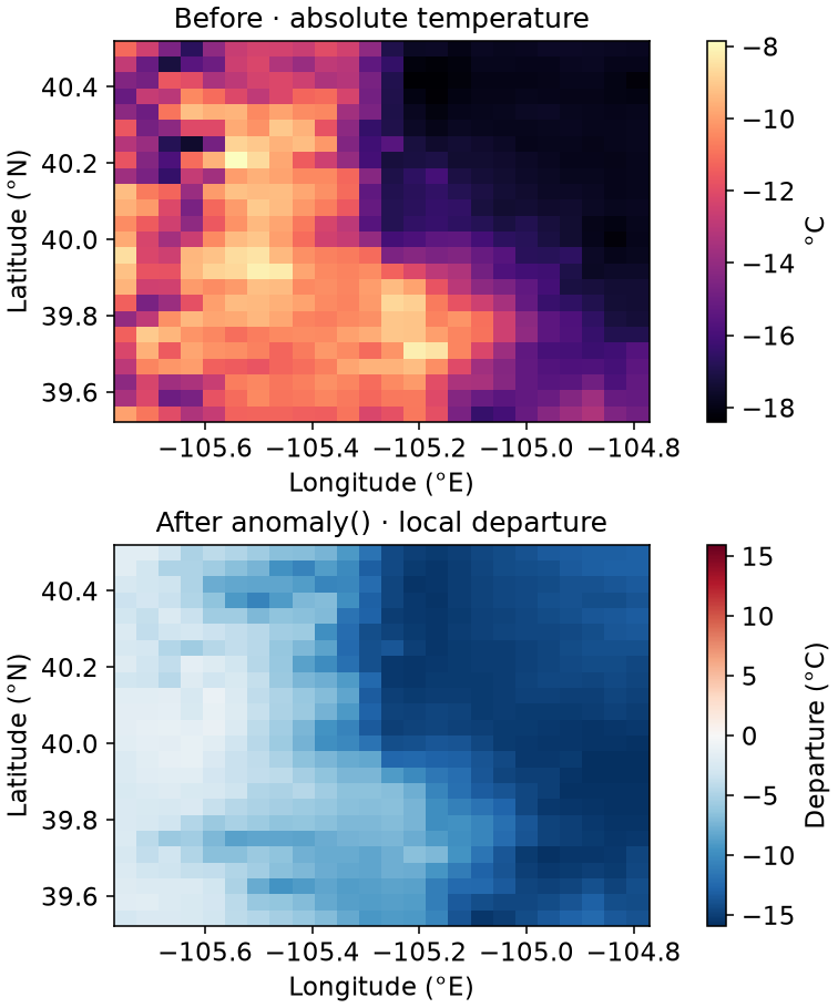
What changed? Negative departures mean colder than that pixel’s baseline. The coldest absolute location need not have the largest departure. A short event-window baseline is not a long-term climate normal.
Summarize region
When was the selected region cold relative to its local baselines?
regional_anomaly = (pipe(departures)
                    | v.mean(dim=("y", "x"), keep_dim=False)).unwrap()
assert regional_anomaly.dims == ("time",)

fig, ax = plt.subplots(figsize=(5.4, 3.4), layout="constrained")
regional_anomaly.plot(ax=ax, marker="o", color="#246b70")
ax.axhline(0, color="0.5", linewidth=0.8)
ax.set(title="After mean() · grid-cell average anomaly", xlabel="Date", ylabel="Departure (°C)")
plt.show()
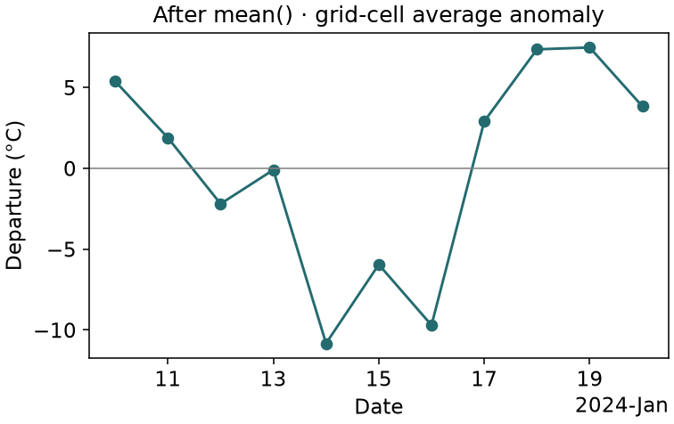
What changed? Space has disappeared from the result, but time remains. This is an equal-cell average on a latitude/longitude grid, not an area-weighted regional estimate.
Compare scales, not units
Does the pipe compute the same z-score as the explicit formula?
standardized = (pipe(window) | v.zscore(dim="time")).unwrap()
direct = (window - window.mean("time")) / window.std("time")
np.testing.assert_allclose(standardized, direct, rtol=1e-6, atol=1e-6)
# Standardization is dimensionless; replace the inherited temperature label.
standardized.attrs["units"] = "1"

fig, axes = plt.subplots(2, 1, figsize=(5.4, 5.8), layout="constrained")
axes[0].hist(window.values.ravel(), bins=24, color="#246b70")
axes[1].hist(standardized.values.ravel(), bins=24, color="#246b70")
axes[0].set(title="Before · selected PRISM values", xlabel="Daily maximum (°C)", ylabel="Cell-days")
axes[1].set(title="After zscore() · per-pixel scaling", xlabel="Standard deviations (unitless)", ylabel="Cell-days")
plt.show()
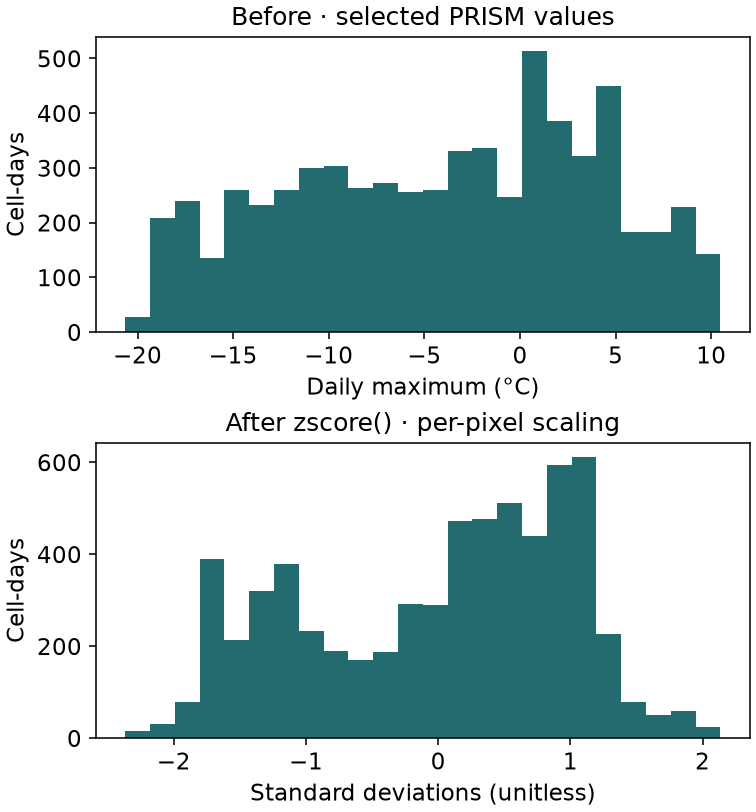
What changed? Each pixel is centered and scaled by its own temporal variability. The pooled histogram is not fitted to a normal distribution, and its cell-days are not independent samples.
Check the saved result
Does explicit NetCDF output preserve the analysis?
from tempfile import TemporaryDirectory
with TemporaryDirectory() as directory:
    target = Path(directory) / "regional_anomaly.nc"
    saved = (pipe(regional_anomaly) | v.to_netcdf(str(target), engine="scipy")).unwrap()
    with xr.open_dataarray(target, engine="scipy") as reopened:
        restored = reopened.load()
    xr.testing.assert_allclose(saved, restored)
    assert restored.attrs["is_synthetic"] == 0
    assert restored.attrs["cubedynamics_metadata_encoding"] == "netcdf-safe-v1"
output_table = pd.DataFrame({
    "Check": ["Dimensions", "Observations", "Values", "Boolean metadata"],
    "Before": [str(saved.dims), str(saved.size), "Reference result", "False"],
    "After reopening": [str(restored.dims), str(restored.size), "Equal (asserted)", "0 · portable flag"],
})

display(output_table)
| Check | Before | After reopening |
|---|---|---|
| Dimensions | ('time',) | ('time',) |
| Observations | 11 | 11 |
| Values | Reference result | Equal (asserted) |
| Boolean metadata | False | 0 · portable flag |
The PRISM regional-anomaly result is written with to_netcdf() and reopened. Numerical equality is asserted while Boolean provenance is intentionally encoded as a portable integer flag; the temporary example file is then removed.
What changed? Export is an explicit side effect. The compact table is more useful here than another identical curve: it reports the tested round trip.
What to learn next
3. Pipes establish order · Verb index · Verb gallery vignette