US Census
Ty Tuff, ESIIL Data Scientist 2023-05-21
The United States Census is an invaluable resource, providing extensive data about the population of the United States, its demographic characteristics, economic activities, and housing characteristics, among other categories. Conducted every ten years, the Census provides a comprehensive snapshot of the country, and is an essential tool for policymakers, researchers, businesses, and anyone seeking to understand more about the nation and its people.
Working with Census data, however, can sometimes be complex due to the sheer size and complexity of the datasets. That’s where the tidycensus package in R comes in. The tidycensus package is a powerful tool that simplifies the process of downloading and working with Census data directly within R, making it easier to access and analyze this rich source of information.
The tidycensus package provides a direct interface to the US Census Bureau’s APIs, allowing users to efficiently load data from the Decennial Census, the American Community Survey (ACS), the Bureau of Economic Analysis (BEA), and other resources directly into R. The returned data is tidy, meaning it’s ready to use with the other packages in the tidyverse ecosystem for data manipulation, analysis, and visualization.
Not only does tidycensus streamline the data retrieval process, but it also helps with other aspects of working with Census data, including handling of Census geographies and variable selection. Moreover, it can return spatial objects that can be easily used for mapping and spatial analysis.
R code:
library(tidycensus)
library(tidyverse)

# Set your Census API key
census_api_key("your_api_key")

# Get the total population for the state of California
ca_pop <- get_acs(
  geography = "state",
  variables = "B01003_001",
  state = "CA"
) %>%
  rename(total_population = estimate) %>%
  select(total_population)

# View the result
ca_pop
R Tidy:
To retrieve census data in R Tidy, we can also use the tidycensus package. Here’s an example of how to retrieve the total population for the state of California using pipes and dplyr functions:
R tidy code:
library(tidycensus)
library(tidyverse)

# Set your Census API key
census_api_key("your_api_key")

# Get the total population for the state of California
ca_pop <- get_acs(
  geography = "state",
  variables = "B01003_001",
  state = "CA"
) %>%
  rename(total_population = estimate) %>%
  select(total_population)

# View the result
ca_pop
Python:
To retrieve census data in Python, we can use the census library. Here’s an example of how to retrieve the total population for the state of California:
Python code:
from census import Census
from us import states
import pandas as pd

# Set your Census API key
c = Census("your_api_key")

# Get the total population for the state of California
ca_pop = c.acs5.state(("B01003_001"), states.CA.fips, year=2019)

# Convert the result to a Pandas DataFrame
ca_pop_df = pd.DataFrame(ca_pop)

# Rename the column
ca_pop_df = ca_pop_df.rename(columns={"B01003_001E": "total_population"})

# Select only the total population column
ca_pop_df = ca_pop_df[["total_population"]]

# View the result
ca_pop_df
Public health example
# example code for downloading poverty measures from the American Community
# Survey through tidycensus and visualizing them through maps
# load the packages we'll use for this section
library(tidycensus)
library(tidyverse)
library(sf)
library(RColorBrewer)
library(mapview)
# download the data from the ACS using the get_acs method from tidycensus
#
# the B05010_002E variable refers to the count of residents who live in
# households with household income below the poverty line; the B05010_001E
# variable refers to the count of residents for whom household income was
# ascertained by the ACS, e.g. the relevant denominator.
#
poverty <- get_acs(
state = 'MA',
county = '025', # this is the FIPS code for Suffolk County, MA
geography = 'tract',
year = 2019, # this indicates the 2015-2019 5-year acs
geometry = TRUE,
variables = c(
in_poverty = 'B05010_002E',
total_pop_for_poverty_estimates = 'B05010_001E')
)
# we're going to recode the variable names to more human-readable names to
# make it easier to work with the data in subsequent steps
poverty <- poverty %>%
mutate(
variable = recode(variable,
# you may notice that tidycensus drops the 'E' from the
# end of the variable code names
B05010_002 = 'in_poverty',
B05010_001 = 'total_pop_for_poverty_estimates'))
# pivot the data wider so that the in_poverty and
# total_pop_for_poverty_estimates; this follows the "tidy" format and approach
# where each row corresponds to an observation.
#
# because the pivot_wider method can mess up your data when your data contains
# geometry/shapefile information, we will remove the geomemtry information
# and add it back in later
poverty_geometry <- poverty %>% select(GEOID) %>% unique() # save the geometry data
poverty <- poverty %>%
sf::st_drop_geometry() %>% # remove geometry data
tidyr::pivot_wider(
id_cols = GEOID,
names_from = variable,
values_from = c(estimate, moe))
# calculate the proportion in poverty
poverty <- poverty %>%
mutate(
proportion_in_poverty = estimate_in_poverty / estimate_total_pop_for_poverty_estimates,
percent_in_poverty = proportion_in_poverty * 100)
# add the geometry back in --
# make sure to merge the data into the sf object with the sf object on the
# left hand side so the output has the sf type including your geometry data
poverty <- poverty_geometry %>%
left_join(poverty)
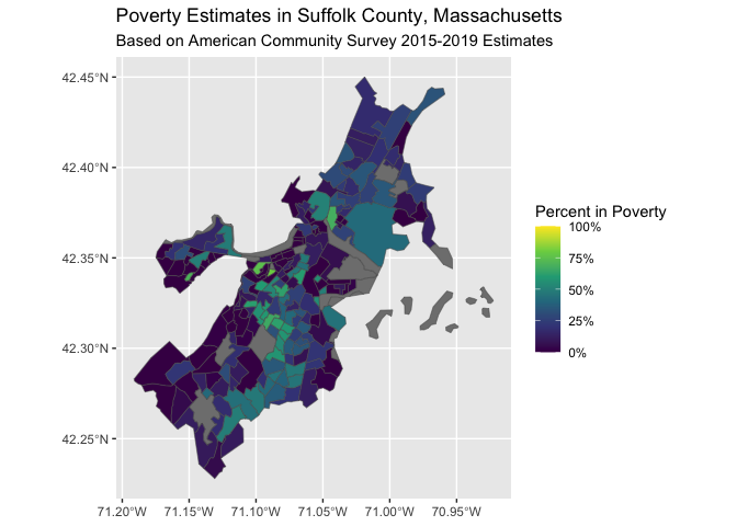
# visualize our point estimates
ggplot(poverty, aes(fill = proportion_in_poverty)) +
geom_sf() +
scale_fill_viridis_c(label = scales::percent_format(),
limits = c(0, 1)) +
labs(fill = "Percent in Poverty") +
ggtitle("Poverty Estimates in Suffolk County, Massachusetts",
subtitle = "Based on American Community Survey 2015-2019 Estimates")
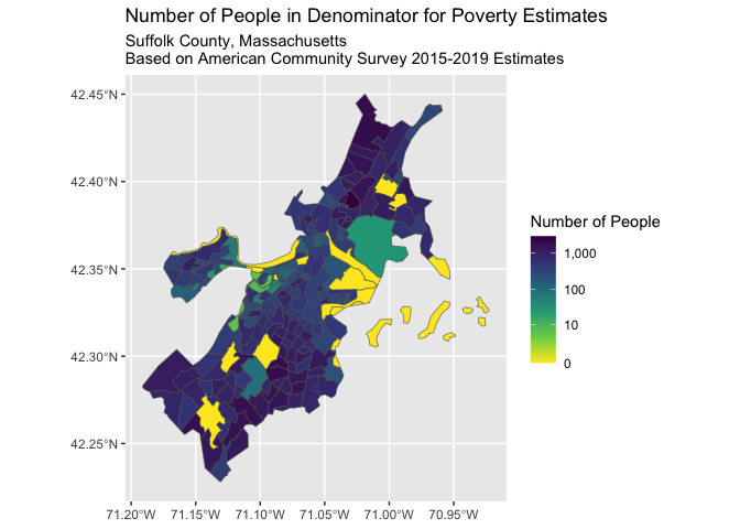
# visualize the denominator counts --
# of significance, note that there are several census tracts where the
# denominator is 0 resulting in NaN estimates for the percent in poverty.
ggplot(poverty, aes(fill = estimate_total_pop_for_poverty_estimates)) +
  geom_sf() +
  scale_fill_viridis_c(label = scales::comma_format(), direction = -1,
                       breaks = c(0, 10, 100, 1000), trans = "log1p") +
  labs(fill = "Number of People") +
  ggtitle("Number of People in Denominator for Poverty Estimates",
          paste0("Suffolk County, Massachusetts\n",
          "Based on American Community Survey 2015-2019 Estimates"))